The Siml Tutorial - Bioreactors
The Siml programming language is a simple domain specific language to solve differential equations. The differential equation are solved numerically. The compiler produces a program in the Python language, that performs the numerical computations. The generated Python program can be used as a stand-alone program, or as a module of a more complex program.
This introduction should teach you enough of the Siml language that you can write simple simulations yourself. The text assumes that you have some experience in writing simple computer programs, and a basic knowledge of differential equations.
The examples are taken from the field of biotechnology.
Example 1: Exponential Growth
Under favorable conditions bacteria grow at a constant (and often fairly fast) rate. If these favorable conditions can be maintained, the newly produced bacteria also grow at the same rate. This results in exponential growth of the bacterial biomass.
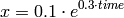
Differential equation (1) describes this behavior. The constant µ is the growth speed.
(1)
With  , and the initial value
  , one can
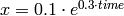
compute a closed-form solution (2). This exact solution
can be used to check the correctness of the numerical solution.
, one can
compute a closed-form solution (2). This exact solution
can be used to check the correctness of the numerical solution.
(2)
The listing below shows a Siml program that computes a numerical solution of differential equation (1).
1 2 3 4 5 6 7 8 9 10 11 12 13 14 15 16 17 | #Simulation of exponential growth
class ExponentialGrowth:
    data x: Float  #Define variable x

    func initialize(this):
        x = 0.1  #Set initial value
solution_parameters(20, 0.1)
func dynamic(this):
$x = 0.3 * x #The differential equation
func final(this):
graph(x, title="Exponential Growth")
print("final-values:", x, time) #For the automatic test script
compile ExponentialGrowth
|
The Exponential Growth program.
The following sections discuss the program in detail:
Comments
Comments start with a # character and extend to the end of the line. The first line of the program contains a comment that covers the whole line. In line three there is a comment that covers only part of the line.
Whitespace
In Siml whitespace is significant, exactly as in the Python language. Statements are grouped by indenting them to a common level. Observe how the four lines starting with: data and func are all indented to the same column. Also observe that the lines immediately following the func statements also have the same indent.
Object Oriented Language
In Siml all simulations are objects [1]. They must have certain main methods, that are invoked during the simulation:
- The initialize method is invoked once at the beginning of the simulation.
- The dynamic method contains the differential equations. It is invoked repeatedly during the simulation.
- The final method is invoked at the end.
class Statement
class ExponentialGrowth:
data x: Float #Define variable x
func initialize(this):
x = 0.1 #Set initial value
Lines 2-6 of the Exponential Growth program.
The class statement defines an object. The simulation object’s name ExponentialGrowth can be freely chosen by the user. The colon : after the name is mandatory. All statements in the body of the simulation object have to be indented to the same level.
data Statement
data x: Float #Define variable x
Line 3 of the Exponential Growth program.
Define the variable x as a floating point number.
The data statement defines attributes (variables, parameters and constants). The data keyword is followed by the attribute’s name (x), a colon :, and the type of attribute (Float).
In Siml attributes have to be defined before they can be used (differently to Python).
| Important built in types | |
|---|---|
| Type | Description |
| Float | Floating point number You will normally use only this type. All other types are only rarely useful. |
| String | Sequence of characters |
| Bool | Logical value |
func Statement
func initialize(this):
Line 5 of the Exponential Growth program.
Here the method initialize is defined.
The func keyword defines functions and methods [2]. It is followed by the method’s name, then comes a parenthesized list of the method’s arguments, followed by a colon (:).
The first argument of a method must always be this, it has exactly the same role as self in Python: It contains the object on which the method operates. Differently to Python you don’t have to write this.x to access the attribute x of the simulation object. Attributes that are accessible through the special argument this are looked up automatically.
All statements in the method’s body must be indented to the same level.
initialize method
    func initialize(this):
        x = 0.1  #Set initial value
        solution_parameters(20, 0.1)
Lines 5-7 of the Exponential Growth program.
The initialize method is invoked once at the beginning of the simulation.
It first computes the initial value of the (state) variable x.
Then the built in function solution_parameters is invoked. It determines the duration of the simulation (20), and the resolution on the time axis (0.1). The simulation always starts at time=0. Therefore the simulation’s variables will be recorded 200 times.
dynamic method
    func dynamic(this):
        $x = 0.3 * x   #The differential equation
Lines 9-10 of the Exponential Growth program.
The dynamic method contains the differential equations. It is invoked many times during the simulation by the solver.
In this simulation, dynamic computes the time derivative of x.
The expression $x denotes the time derivative. The dollar($) operator is multi functional: it accesses the time derivative, and it also tells the compiler that a variable is a state variable [3].
final method
    func final(this):
        graph(x, title="Exponential Growth")
        print("final-values:", x, time) #For the automatic test script
Lines 12-14 of the Exponential Growth program.
The final method is invoked at the end of the simulation.
In this simulation proigram is creates a graph of the variable x versus time with the built in graph function. Then it sends a short text to the standard output with the built in print function. The text contains the final values of x and time.
compile statement
compile ExponentialGrowth
Line 17 of the Exponential Growth program.
Tell the compiler to compile the object ExponentialGrowth.
The keyword compile is followed by the (class) name of the simulation object. There can be multiple compile statements in one file.
Running the Simulation
The Exponential Growth program is available on the website, and in the *.tar.gz and *.zip archives as models/biological/exponential_growth.siml
The simulation program can be typed into any text editor. For details on editors see: Editors.
If you have saved the Exponential Growth program under the name exponential_growth.siml you can compile and run the program at once by typing the following into a shell window:
$> simlc exponential_growth.siml -r all
When run, the simulation opens a window with a graph similar to the one below.
The graph matches the exact solution (2)
( ) very well.
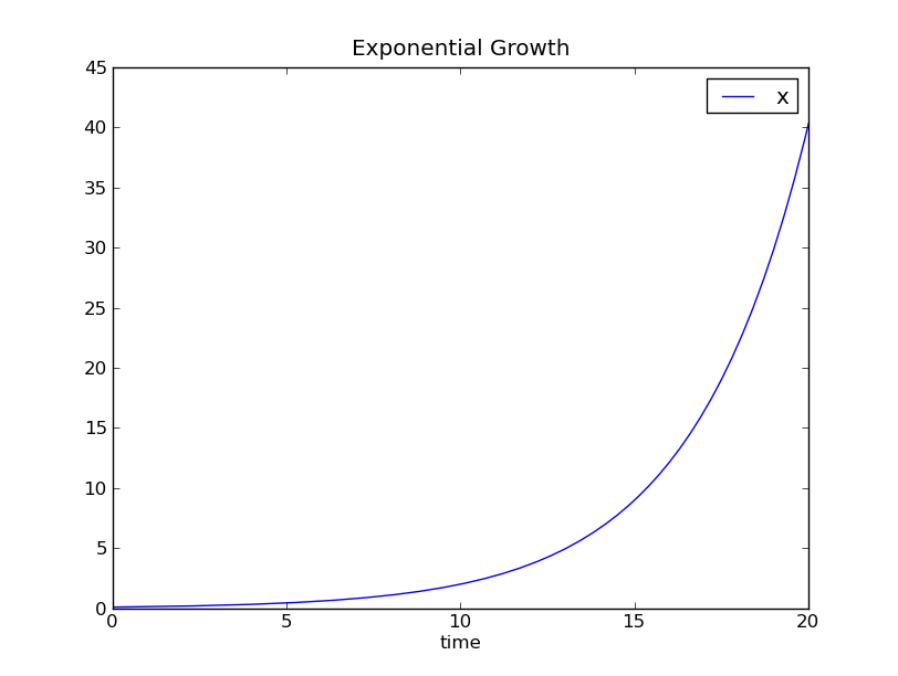
Biomass concentration versus simulation time.
Example 2: Batch Reactor
The second example is more complex as well as more detailed. It consists of two coupled differential equations, both are non linear. The bacteria this time live in a batch reactor. This is a container which is initially full of nutrient broth, and a small initial amount of bacteria. While the bacteria multiply in the reactor, they consume the nutrients until there are none left. In the end there is a high concentration of bacteria in the reactor and a low concentration of nutrients.
The simulation does not simulate the size of the reactor, only the concentrations of bacteria and nutrients. The reactor could be a shaking flask as well as a big tank.
The simulation has two state variables: X the concentration of biomass, and S the concentration of nutrients (usually called substrate). The growth speed µ is an algebraic variable.
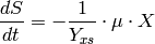
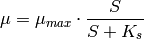
The growth of the bacteria is described by equation (3); the nutrient consumption is described by equation (4). The growth speed of the biomass (5) is dependent on the nutrient concentration.
(3)
(4)
(5)
SIML Program
This SIML program solves the system of differential equations. The initial values and parameters are realistic values for Corynebacterium Glutamicum growing on lactate.
1 2 3 4 5 6 7 8 9 10 11 12 13 14 15 16 17 18 19 20 21 22 23 24 25 26 27 28 29 30 31 32 33 | #Biological reactor with no inflow or outflow
class Batch:
#Define values that stay constant during the simulation.
data mu_max, Ks, Yxs: Float param
#Define values that change during the simulation.
data mu, X, S: Float
#Initialize the simulation.
    func initialize(this):
        #Specify options for the simulation algorithm.
        solution_parameters(duration=20, reporting_interval=0.1)
        #Give values to the parameters
        mu_max = 0.32 #[1/h] max growth speed
        Ks     = 0.01 #[g/l] at this lactate concentration growth speed is 0.5*mu_max
        Yxs    = 0.5  #[g/g] one g lactate gives this much biomass
        #Give initial values to the state variables.
        X      = 0.1  #[g/l] initial biomass concentration
        S      = 20   #[g/l] initial sugar concentration
#compute dynamic behavior - the system's 'equations'
    func dynamic(this):
        mu = mu_max * S/(S+Ks) #growth speed (of biomass) [1/h]
        $X = mu*X              #change of biomass concentration [g/l/h]
        $S = -1/Yxs*mu*X       #change of sugar concentration [g/l/h]
#show results
    func final(this):
        graph(mu, X, S, title="Batch Reactor");
        #For the test scripts
        print("final-values:", X, S, time)
compile Batch
|
Program Overview
Again, the simulation object is defined with a class statement.
First the simulation’s data attributes are defined:
- In line 4 so called parameters are defined. These attributes stay constant during the simulation, but they can change in between simulations.
- In line 6 the variables are defined, these attributes change during the simulation. The recorded values of X and S are the solution of the differential equation.
In Lines 9 - 30 the simulation object’s methods are defined. Simulation objects must have certain main methods, that are called by the run time library during the simulation:
- The initialize method is called once at the beginning of the simulation.
- The dynamic method contains the differential equations. It is called repeatedly during the simulation.
- The final method is called at the end.
Finally the compile statement tells the compiler to create code for the class Batch. The compiler creates a Python class for the Siml class Batch.
Attribute Roles
Attributes of a simulation object have one of three different roles. These roles are selected by putting a modifier keyword after the type in the data statement:
- Constants are known at compile time, and don’t change at all. The compiler computes expressions with constants at compile time; therefore constants may not appear in the compiled program. Constants are defined with the modifier const.
- Parameters stay constant during the simulation, but they can change in between simulation runs. They are defined with the modifier param.
- Variables change during the simulation. The recorded values of the state variables versus simulation time, are the solution of the differential equation. Class attributes without modifiers become variables; however they can be defined with the optional modifier variable.
| Roles for attributes in Siml | ||
|---|---|---|
| Role | Keyword | Description |
| Constant | const | Attributes that are known at compile time. |
| Parameter | param | Constant during the simulation run, but can change in between simulations. |
| Variable | variable | Attributes that vary during the simulation. Modifier is optional. |
initialize Method
func initialize(this):
#Specify options for the simulation algorithm.
solution_parameters(duration=20, reporting_interval=0.1)
#Give values to the parameters
mu_max = 0.32 #[1/h] max growth speed
Ks = 0.01 #[g/l] at this lactate concentration growth speed is 0.5*mu_max
Yxs = 0.5 #[g/g] one g lactate gives this much biomass
#Give initial values to the state variables.
X = 0.1 #[g/l] initial biomass concentration
S = 20 #[g/l] initial sugar concentration
Lines 9-18 of the Batch simulation.
The initialize method is called at the beginning of the simulation run. Its purpose is to compute parameters and initial values, as well as to configure the solver.
In this example the solver is configured first, which is done with the built in function solution_parameters. The duration of the simulation is set to 20, the time between data points is set to 0.1.
Then the values of the parameters ( ) are determined.
Finally the initial values of the state variables (
) are determined.
Finally the initial values of the state variables ( ) are determined.
The algebraic variable
) are determined.
The algebraic variable  does not need an initial value.
dynamic Method
func dynamic(this):
mu = mu_max * S/(S+Ks) #growth speed (of biomass) [1/h]
$X = mu*X #change of biomass concentration [g/l/h]
$S = -1/Yxs*mu*X #change of sugar concentration [g/l/h]
Lines 21-24 of the Batch simulation.
The dynamic method is called repeatedly during the simulation by the solver algorithm. It computes the time derivatives of the state variables.
As Siml has imperative semantics, mu has to be computed first [4]. Also because of these imperative semantics the equal (=) operator really is an assignment. On the left hand side of the equal operator there must always be just an attribute. All attributes can only be assigned once; no assigned value can ever be changed.
final Method
func final(this):
graph(mu, X, S, title="Batch Reactor");
#For the test scripts
print("final-values:", X, S, time)
Lines 27-30 of the Batch simulation.
The final method is called at the end of the simulation, its purpose is to display or store the simulation results. All variables have the values that were computed for the last point in time.
In this example a graph of the variables µ, X and S is produced. Then a line of text is written to the standard output, which contains the final values of X, S and time.
| Built in functions for use in the final method. | |
|---|---|
| Name | Description |
| graph (*args, title="") | Display graph of (possibly multiple) variables versus time. |
| save (file_name) | Save simulation results into a file. |
| print (*args, area="",end="\n") | Output text. |
Running the Simulation
The program for the batch reactor is available on the website, and in the *.tar.gz and *.zip archives as models/biological/bioreactor_simple.siml
The simulation program can be typed into any text editor. For details on editors see: Editors.
If you have saved the program under the name bioreactor_simple.siml you can compile and run the program at once by typing the following into a shell window:
$> simlc bioreactor_simple.siml -r all
At the end of the simulation a window opens, that shows the simulation results:
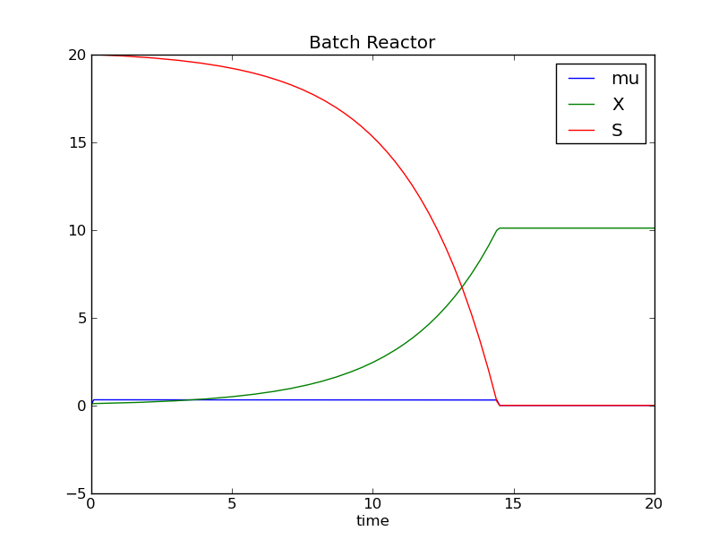
Graph of X, S and mu, versus simulation time.
Editors
A program in the Siml language can be typed into any text editor. If the editor has syntax highlighting, choose Python highlighting which works reasonably well for Siml.
For editors based on the Kate Part ( Kate, Kwrite, Kdevelop) there is a special highlight file for Siml available: hl_siml.xml. To copy this file to the Kate Part’s highlight directory run the script hl_install (in a shell window).
$> ./hl_install
Footnotes
| [1] | In this respect Siml is similar to the Java programming language. |
| [2] | You may call methods member functions in Siml, because there are some deliberate similarities to the C++ programming language: The special this argument (which is hidden in C++) that contains a refference to the current object, and the automatic attribute lookup through this. |
| [3] | The dollar operator really has three functions: it accesses the time derivative; it marks a variable as a state variable; and it creates a place to store the time derivative (if necesary). The time derivative is just an other variable, but usually it can only be accessed by the $ operator. |
| [4] | Statement reordering is a planned feature, but it is unclear if it would cause much confusion for relative little gain in convenience. |